First Play With SOM and GSOM
We
recommend to look on the “First Play With PCA” tutorial before you
start this play with SOM and GSOM.
Click
on the “Data set” button
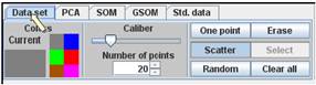
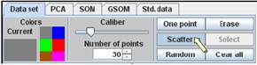
Use
the “Scatter” button with various “Caliber” and “Number of points” values; in
addition, you may add several random points using the button “Random”.
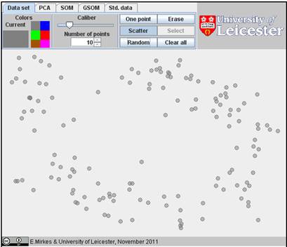
Prepare
a cloud of data points. We prepared a data cloud that slightly resembles a horseshoe:
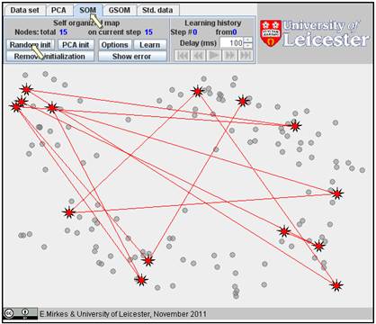
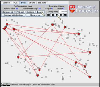
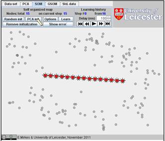
Go
to “SOM” and click the “Random init.” button several times (we used 15 times).
This is the random initiation of SOM: 15 initial positions of coding vectors
are randomly selected at data points:
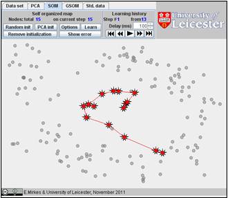
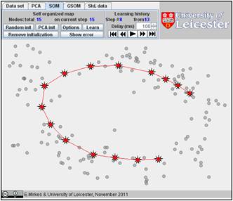
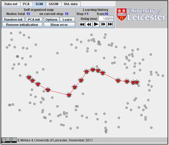
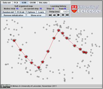
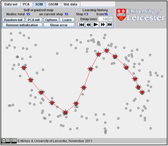
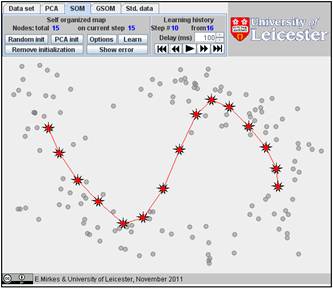
Click
on the “Learn” button. After learning, everybody would like to see the result.
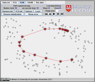
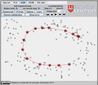
Go to the “Learning history”. The history of iterations will be demonstrated
step by step. There are 13 steps in the history with the final result at the
end. Below, after the random initiation, the steps 1, 2, 3, 8, and 13 are
presented below.
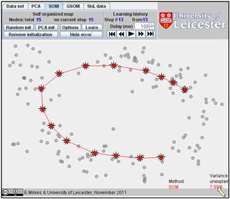
You
can use the “Show error” button and find the value of FVU in the right bottom
corner. Here it is 7.99%.
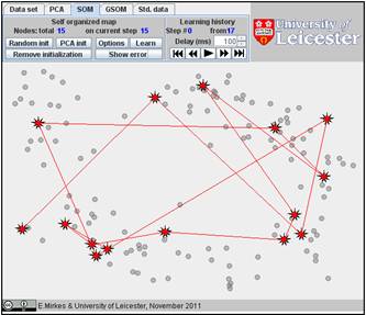
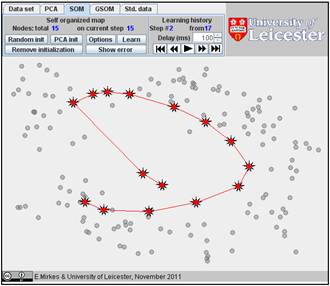
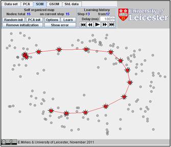
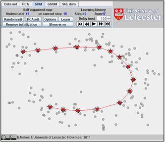
The
result depends on the initial position. You can change the initiation for the
same data set, just push the “Remove initiation” button. When we started from
another random initiation with the same amount of points (15), we got
significantly different result. The story is presented below. There are 17
steps in the history. We represent the random initiation and the steps 1, 2, 3,
9, and 17:
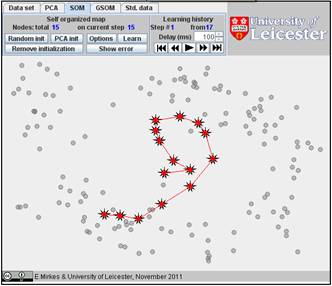
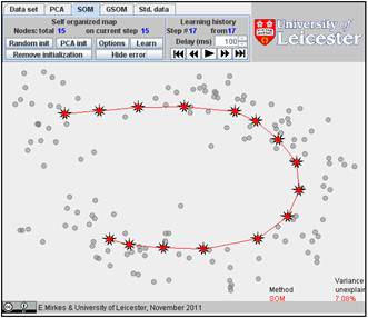
The
value of FVU for this approximation is a bit better than for the previous one,
7.08% versus 7.99%. It may be useful to try several initial approximations and
select the result with the smallest FVU. Can you do this?
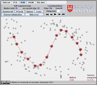
You
can also select the PCA initialization, just click several times on the “PCA
init” button. We generated the PCA initiation for the same number of points
(15) and found SOM. The history is below. There are 16 steps in the history,
and we present here steps 1, 2, 3, 10, and 16. The FVU for this initiation is
10.31 which is significantly worse than for the previous examples of the random
initiation. (Sometimes, for other data sets, the PCA initialization can work
better.)
A research task. Efficiency of the
PCA initiation: a myth or reality. You can
often read that PCA initiation of SOM is better. Of course, one benefit is
obvious. It is reproducibility: if you start SOM learning from the PCA initiation
with the same number of points uniformly distributed along the first principal
component with the same variance then the result does not change. But it is not
obvious that the PCA initiation is better for approximation. Moreover, random
initiation gives the possibility to generate several different SOMs and then
select the best. Try to compare systematically different types of initiations
on various data sets. It may be useful to use the Std. data collections. (We
recommend you to try Spiral 2 that is a not very difficult but not trivial
learning example.)
**********************
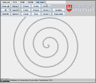
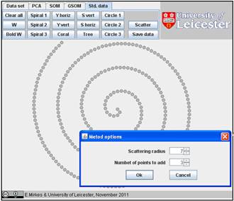
You
can explore the approximation ability of 1D SOMs on various sets from the Std.
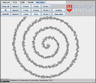
data collections. Let us try “Spiral 1”; this is a rather difficult task. We will
study, how the accuracy of approximation depends on the number of points. Let
us go to “Std. data”, “Clear all”, and “Spiral 1” (below). For smearing the
image we go to “Scatter” and select the Scattering radius 7 and the Number of
points to add 3. After we press OK, the smeared spiral appears.
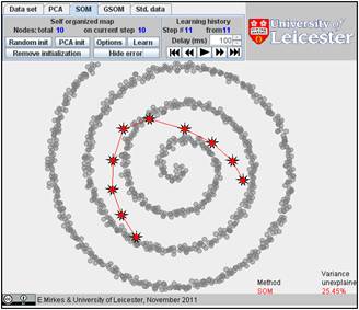
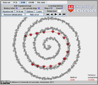
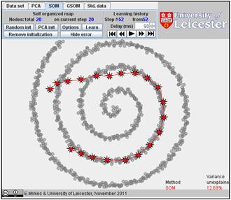
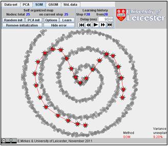
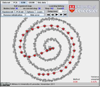
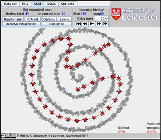
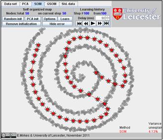
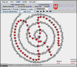
We
initiated SOM with various numbers of nodes and, after learning, got the
following results. Nine configurations are below.
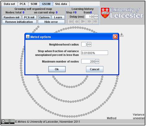
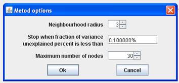
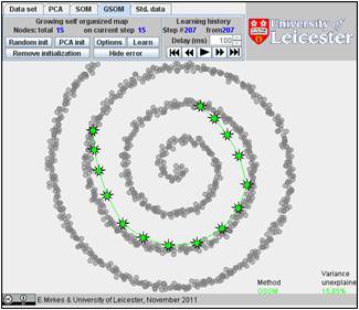
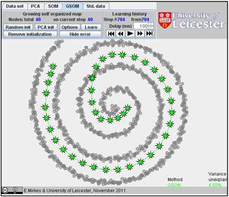
It
is interesting to compare SOM and GSOM on this example. To stop GSOM at the
given number of points, you can select in GSOM/Options a high accuracy of
approximation (0.1% or 0.01%) and the desired number of points (see below). For
reproducibility, it is recommended to start from one point (the first learning
iteration will move to the mean point).
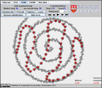
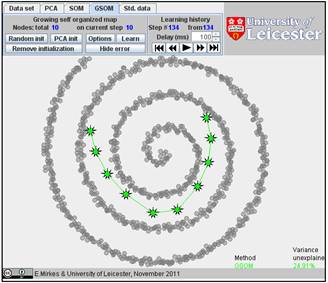
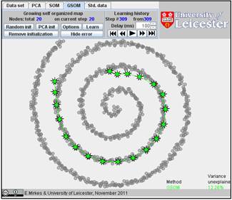
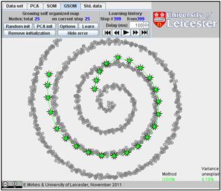
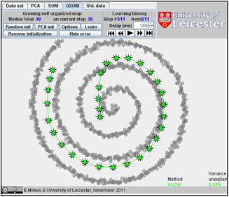
Below
are the learning results for the same numbers of points in GSOM as for the SOMs
above. The picture of approximation for GSOM looks more attractive than for SOM
but the accuracy of approximation (see in Table) is approximately the same.
Table. FVU for presented examples of SOM and GSOM with various numbers of
nodes.
|
Number
of nodes |
10 |
15 |
20 |
25 |
30 |
40 |
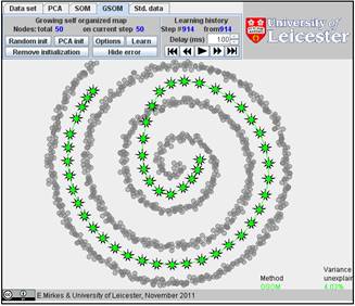
50 |
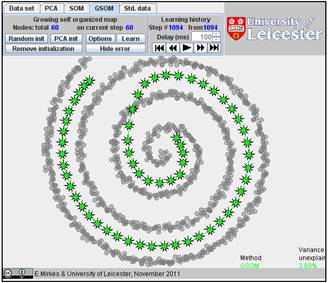
60 |
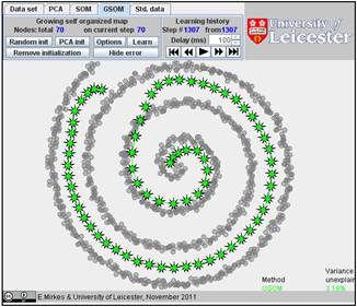
70 |
|
FVU
for SOM |
25.45% |
15.59% |
12.09% |
9.20% |
6.42% |
5.09% |
4.13% |
3.62% |
2.63% |
|
FVU
for GSOM |
24.91% |
15.85% |
12.26% |
9.19% |
6.99% |
4.58% |
4.03% |
3.68% |
3.19% |
If
the learning history is too long then to speed the slideshow you are welcome to
reduce the delay time (in the “Delay” window) to the minimal value 10 ms.
Research task. Find for Spiral 1, for what number of nodes GSOM becomes stably better
than SOM. Can you perform a detailed
and scientifically sound study?
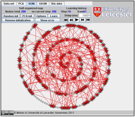
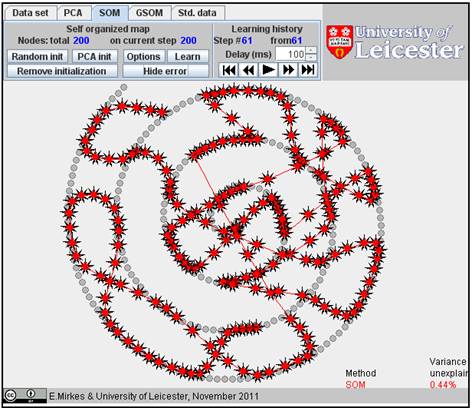
For
example, the 200 nodes approximation of Spiral 1 by GSOM is almost 10 times
better than the approximation by SOM (see the results below, for 200 SOM nodes
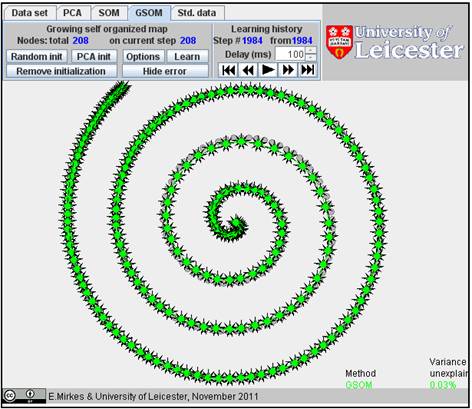
FVU=0.44% and for 200 GSOM nodes FVU=0.05%). For 208 nodes, FVU for GSOM
becomes 0.03% and geometrically this approximation looks perfect.